Multiple Concurrent Downloads using RCurl

Overview

In this example, we look at how we can send multiple HTTP requests and process them concurrently. The basic idea is this. We specify a collection of URIs to download when establishing the HTTP requests, but don't send any of the requests until they are all constructed. Then, we send the requests and harvest the results. When the last one finishes, we return control to the caller.

This is different from processing the requests in the background. In that case, having dispatched the requests, control would be returned to the caller and R would be able to do other things. Notification of pending content from the request would be done via the event loop. This is feasible (at least on Unix), but different from the example we are describing here.

The Basics

The implementation requires using the multi interface for libcurl. We create a multi handle and then we create a regular curl handle for each individual request, i.e. for each URI to be fetched. We add each of these regular/easy curl handles to the multi handler and then call curlMultiPerform() until it terminates. Terminating means either an error or that each of the requests has completed.


getURIs =
function(uris, ..., multiHandle = getCurlMultiHandle(), .perform = TRUE)
{
  content = list()
  curls = list()

  for(i in uris) {
    curl = getCurlHandle()
    content[[i]] = basicTextGatherer()
    opts = curlOptions(URL = i, writefunction = content[[i]]$update, ...)    
    curlSetOpt(.opts = opts, curl = curl)
    multiHandle = push(multiHandle, curl)
  }

  if(.perform) {
     complete(multiHandle)
     lapply(content, function(x) x$value())
   } else {
     return(list(multiHandle = multiHandle, content = content))
   }
}

To test this, we can fetch pages from the Omegahat Web site:


getURIs(c("http://www.omegahat.org/index.html", "http://www.omegahat.org/RecentActivities.html"))

To see what effect we have on timing, let's run the asynchronous version and the serial version and compute their times.


uris = c("http://www.omegahat.org/index.html", "http://www.omegahat.org/RecentActivities.html")

atime = system.time(z <- getURIs(uris))
stime = system.time(zz <- lapply(uris, getURL))

How does this vary with larger numbers of URIs?


uris = c("http://www.omegahat.org/index.html", 
         "http://www.omegahat.org/RecentActivities.html",
         "http://www.omegahat.org/RCurl/index.html", 
         "http://www.omegahat.org/RCurl/philosophy.xml",
         "http://www.omegahat.org/RCurl/philosophy.html")

atime = system.time(z <- getURIs(uris))
stime = system.time(zz <- lapply(uris, getURL))

The key thing to note is that the user and system CPU times are much lower for the serialized downloads, but the overall elapsed time is significantly higher. This is quite reasonable when one thinks about it. The asynchronous version spends time switching between the downloads, checking if there is anything to be read on each. The serialized version does not have to do this switching but can focus on each single download. The switch is done in a call to select. This can be arranged not to consume CPU time, if I recall correctly, but it will do so if a timeout is specified.

This tradeoff between elapsed time and CPU time is a convenient one. The user can chose which is important for their particular situation.

Being statisticians, we should repeat the measurement process and get data about the variability of the times taken in each approach.

atimes = sapply(1:40, function(i) system.time(getURI(uris)))
stimes = sapply(1:40, function(i) system.time(getURI(uris, async = FALSE)))

times = data.frame(user = c(atimes[1,], stimes[1,]),
                   system = c(atimes[2,], stimes[2,]),
                   elapsed = c(atimes[3,], stimes[3,]),
                   style = factor(c(rep("Asynchronous", 40), rep("Serial", 40))))


by(times, times$style, summary)

times$style: Asynchronous
      user           system          elapsed               style   
 Min.   :0.340   Min.   :0.0300   Min.   :0.430   Asynchronous:40  
 1st Qu.:1.665   1st Qu.:0.1275   1st Qu.:2.085   Serial      : 0  
 Median :2.135   Median :0.1700   Median :2.865                    
 Mean   :2.319   Mean   :0.1790   Mean   :3.091                    
 3rd Qu.:2.740   3rd Qu.:0.2025   3rd Qu.:3.683                    
 Max.   :5.780   Max.   :0.5400   Max.   :7.410                    
------------------------------------------------------------ 
times$style: Serial
      user            system           elapsed                style   
 Min.   :0.0500   Min.   :0.00000   Min.   : 1.780   Asynchronous: 0  
 1st Qu.:0.0875   1st Qu.:0.00750   1st Qu.: 3.788   Serial      :40  
 Median :0.1050   Median :0.01000   Median : 5.320                    
 Mean   :0.1168   Mean   :0.01325   Mean   : 5.973                    
 3rd Qu.:0.1225   3rd Qu.:0.02000   3rd Qu.: 7.875                    
 Max.   :0.2500   Max.   :0.04000   Max.   :14.020

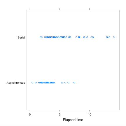
As usual, a picture makes things clearer. A stripplot() of elapsed time shows us the different distributions for the serial and asynchronous transfer.

Clearly, the download times for the asynchronous download are significantly shorter than for the serial download. And the variability is also much larger.

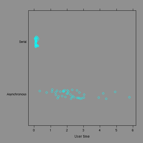
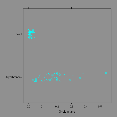
Stripplots for user and system times show the difference between the two modes of downloading also and that the asynchronous method makes more use of system resources.

library(RCurl)